The Optimal Bayes Classifier: Bivariate Case

8 min read Published on 16 Nov 2024

#Probability #Bayes Classifier #Bayes Theorem #R #Multivariate Statistics

Introduction

In a previous post, we explored the Optimal Bayes Classifier for univariate distributions. Here, we extend this framework to bivariate distributions, where we classify observations based on two features simultaneously. This extension allows us to capture relationships between features and provides a more realistic modeling approach for many classification problems.

We maintain the same fundamental assumption: $X$ and $Y$ have a joint distribution $P_{X,Y}$ , and $\{X_i, Y_i\}_{i=1}^{n}$ represents a random sample from this distribution. However, now $X = (X_1, X_2)$ is a bivariate random vector, and we seek to classify based on both components.

Suppose we want to classify whether a test subject has stress based on two brain activity measurements:

$X_1$ : Average brain activity in the Amygdala
$X_2$ : Average brain activity in the Prefrontal Cortex
$Y$ : 1 if the subject has stress (red), and 0 if not (green)

The Bivariate Bayes Classifier

The classification rule remains the same as in the univariate case:

\begin{equation} f(X) = \arg\max_{Y=y}P(Y=y | X_1=x_1, X_2=x_2) \end{equation}

Using Bayes’ Theorem, we can rewrite this as:

\begin{equation} f(X) = \arg\max_{Y=y}P(X_1=x_1, X_2=x_2|Y=y)P(Y=y) \end{equation}

Multivariate Normal Distribution

For the bivariate case, we model the conditional distribution of the inputs as a bivariate normal distribution:

P(X_1, X_2|Y=y) \sim \text{MVN}(\boldsymbol{\mu}_y, \boldsymbol{\Sigma}_y)

where $\boldsymbol{\mu}_y = (\mu_{y1}, \mu_{y2})$ is the mean vector and $\boldsymbol{\Sigma}_y$ is the covariance matrix for class $y$ .

The probability density function of a bivariate normal distribution is:

f(x_1, x_2) = \frac{1}{2\pi\sqrt{|\boldsymbol{\Sigma}|}} \exp\left(-\frac{1}{2}(\mathbf{x} - \boldsymbol{\mu})^T \boldsymbol{\Sigma}^{-1} (\mathbf{x} - \boldsymbol{\mu})\right)

where $\mathbf{x} = (x_1, x_2)^T$ and $|\boldsymbol{\Sigma}|$ denotes the determinant of the covariance matrix.

Decision Boundary

The decision boundary in the bivariate case occurs when:

P(Y=1|X_1=x_1, X_2=x_2) = P(Y=0|X_1=x_1, X_2=x_2)

This leads to:

\begin{equation} \frac{P(X_1=x_1, X_2=x_2|Y=1)P(Y=1)}{P(X_1=x_1, X_2=x_2|Y=0)P(Y=0)} = 1 \end{equation}

Unlike the univariate case, the decision boundary in the bivariate case is typically a curve (or surface in higher dimensions) rather than a single point. When the covariance matrices are equal ( $\boldsymbol{\Sigma}_0 = \boldsymbol{\Sigma}_1$ ), the decision boundary is linear. When they differ, the boundary becomes quadratic.

Computing the Decision Boundary

The decision boundary is computed numerically using a grid-based approach. The method consists of four main steps:

Create a grid: Generate a fine grid of points $(x_1, x_2)$ covering the region of interest. In the R code, this is done with:

x1_range <- seq(min(sim_df$x1) - 0.5, max(sim_df$x1) + 0.5, length.out = 200)
x2_range <- seq(min(sim_df$x2) - 0.5, max(sim_df$x2) + 0.5, length.out = 200)
grid <- expand.grid(x1 = x1_range, x2 = x2_range)

This creates a 200×200 grid (40,000 points total) covering the data range.

Compute probabilities (vectorized): For all grid points simultaneously, calculate both posterior probabilities using vectorized operations with dmvnorm():

grid$prob_class0 <- dmvnorm(grid[, c("x1", "x2")], 
                            mean = mu0, 
                            sigma = sigma0) * (1 - theta)
 
grid$prob_class1 <- dmvnorm(grid[, c("x1", "x2")], 
                            mean = mu1, 
                            sigma = sigma1) * theta

This vectorized approach is much more efficient than computing probabilities point-by-point in a loop.

Find the boundary: The decision boundary consists of all points where $P(Y=1|X) = P(Y=0|X)$ , or equivalently, where $P(Y=1|X) - P(Y=0|X) = 0$ . The code computes this difference:
```
grid$prob_diff <- grid$prob_class1 - grid$prob_class0
```
Visualize using contours: The boundary is visualized as a contour line where the difference equals zero:
```
geom_contour(data = grid, 
             aes(x = x1, y = x2, z = prob_diff), 
             breaks = 0, color = "#34495E", linewidth = 2)
```
The breaks = 0 argument tells ggplot2 to draw only the contour where $z = 0$ , which corresponds to the decision boundary.

This numerical method works for both equal and unequal covariance matrices, providing a smooth visualization of the decision boundary without requiring analytical solutions.

Example

In the context of stress classification, suppose we know that:

$Y \sim \text{Bernoulli}(\theta = 0.3)$
$(X_1, X_2)|Y=0 \sim \text{MVN}(\boldsymbol{\mu}_0 = (5, 3), \boldsymbol{\Sigma}_0)$
$(X_1, X_2)|Y=1 \sim \text{MVN}(\boldsymbol{\mu}_1 = (7, 5), \boldsymbol{\Sigma}_1)$

where the covariance matrices are:

\boldsymbol{\Sigma}_0 = \boldsymbol{\Sigma}_1 = \begin{pmatrix} 1 & -0.3 \\ -0.3 & 1 \end{pmatrix}

The negative correlation ( $-0.3$ ) indicates that when one brain region is highly active, the other tends to be less active, which is a realistic biological pattern.

The Classifier

For a given observation $\mathbf{x} = (x_1, x_2)$ , the classifier computes:

f(\mathbf{x}) = \arg\max_{y \in \{0,1\}} \frac{1}{2\pi\sqrt{|\boldsymbol{\Sigma}_y|}} \exp\left(-\frac{1}{2}(\mathbf{x} - \boldsymbol{\mu}_y)^T \boldsymbol{\Sigma}_y^{-1} (\mathbf{x} - \boldsymbol{\mu}_y)\right) \theta^{y}(1-\theta)^{1-y}

Visualizing the Decision Boundary

The decision boundary can be visualized as a contour line where the probabilities of both classes are equal. Figure 1 shows the simulated data points with their true class labels, along with confidence ellipses and the decision boundary.

Bivariate Bayes Classifier

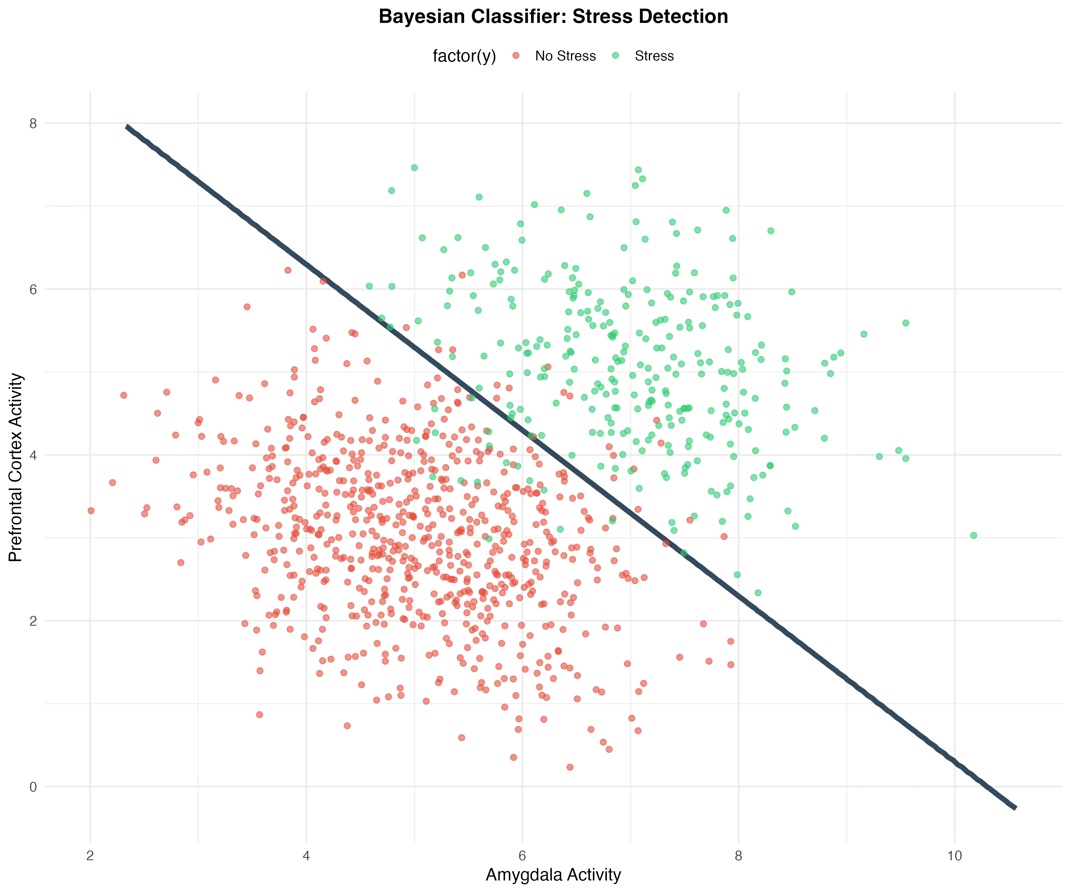
Figure 1: Bayesian Classifier for stress detection. The dark blue curve represents the decision boundary where $P(Y=1|X) = P(Y=0|X)$ .

Key Differences from the Univariate Case

Decision Boundary: In the univariate case, the decision boundary is a single point. In the bivariate case, it’s a curve (or surface in higher dimensions).
Covariance Structure: The bivariate case allows us to model correlations between features, which can significantly impact classification performance.
Visualization: While univariate distributions can be visualized with simple line plots, bivariate distributions require contour plots, scatter plots, or heatmaps.
Computational Complexity: The bivariate case requires matrix operations (inverses, determinants) which are more computationally intensive than the univariate case.

Conclusions

The bivariate extension of the Bayes Classifier demonstrates how the framework naturally generalizes to higher dimensions. The decision boundary becomes more complex, and we can capture relationships between features through the covariance structure.

As future work, we can:

Explore cases where $\boldsymbol{\Sigma}_0 \neq \boldsymbol{\Sigma}_1$ (quadratic decision boundaries)
Extend to higher-dimensional multivariate distributions
Investigate the impact of different covariance structures on classification performance
Compare the bivariate Bayes Classifier with other multivariate classification methods

R Code

library(ggplot2)
library(MASS)      # Para mvrnorm
library(mvtnorm)   # Para dmvnorm
 
## ============================================================
## 1. CONFIGURACIÓN Y GENERACIÓN DE DATOS
## ============================================================
 
set.seed(123)  # Para reproducibilidad
 
theta <- 0.3
y <- rbinom(1000, 1, theta)
n1 <- sum(y == 1)
n2 <- sum(y == 0)
 
## Parámetros de las distribuciones
mu0 <- c(5, 3)
sigma0 <- matrix(c(1, -0.3, -0.3, 1), nrow = 2)
 
mu1 <- c(7, 5)
sigma1 <- matrix(c(1, -0.3, -0.3, 1), nrow = 2)
 
## Generar datos simulados
xy0 <- mvrnorm(n2, mu0, sigma0)
xy1 <- mvrnorm(n1, mu1, sigma1)
sim_df <- data.frame(rbind(cbind(xy0, 0), cbind(xy1, 1)))
colnames(sim_df) <- c("x1", "x2", "y")
 
## ============================================================
## 2. CALCULAR DECISION BOUNDARY (MÉTODO VECTORIZADO)
## ============================================================
 
x1_range <- seq(min(sim_df$x1) - 0.5, max(sim_df$x1) + 0.5, length.out = 200)
x2_range <- seq(min(sim_df$x2) - 0.5, max(sim_df$x2) + 0.5, length.out = 200)
grid <- expand.grid(x1 = x1_range, x2 = x2_range)
 
## Calcular probabilidades (vectorizado - muy eficiente)
grid$prob_class0 <- dmvnorm(grid[, c("x1", "x2")], 
                            mean = mu0, 
                            sigma = sigma0) * (1 - theta)
 
grid$prob_class1 <- dmvnorm(grid[, c("x1", "x2")], 
                            mean = mu1, 
                            sigma = sigma1) * theta
 
grid$prob_diff <- grid$prob_class1 - grid$prob_class0
 
## ============================================================
## 3. GRÁFICO 1: PUNTOS CON DECISION BOUNDARY
## ============================================================
 
p1 <- ggplot() +
  
  geom_contour(data = grid, 
               aes(x = x1, y = x2, z = prob_diff), 
               breaks = 0, 
               color = "#34495E", 
               linewidth = 2) +
  
  geom_point(data = sim_df, 
             aes(x = x1, y = x2, color = factor(y)), 
             alpha = 0.6, 
             size = 2) +
  
  scale_color_manual(
    values = c("0" = "#E74C3C", "1" = "#2ECC71"),
    labels = c("No Stress", "Stress"),
    name = ""
  ) +
  
  labs(
    title = "Bayesian Classifier: Stress Detection",
    x = "Amygdala Activity",
    y = "Prefrontal Cortex Activity"
  ) +
  
  theme_minimal(base_size = 14) +
  theme(
    plot.title = element_text(face = "bold", size = 16, hjust = 0.5),
    legend.position = "top",
    panel.background = element_rect(fill = "white", color = NA),
    plot.background = element_rect(fill = "white", color = NA)
  )
 
print(p1)
ggsave("bayes_classifier_boundary.png", p1, width = 10, height = 8, dpi = 300)
 
## ============================================================
## 4. GRÁFICO 2: HEATMAP DE PROBABILIDADES
## ============================================================
 
p2 <- ggplot(grid, aes(x = x1, y = x2, fill = prob_diff)) +
  
  geom_tile() +
  
  scale_fill_gradient2(
    low = "#E74C3C", 
    mid = "white", 
    high = "#2ECC71",
    midpoint = 0, 
    name = "P(Y=1|X) - P(Y=0|X)"
  ) +
  
  geom_contour(aes(z = prob_diff), 
               breaks = 0, 
               color = "#3498DB",
               linewidth = 1.5) +
  
  geom_point(data = sim_df, 
             aes(x = x1, y = x2, color = factor(y)), 
             inherit.aes = FALSE,
             alpha = 0.8, 
             size = 1.2) +
  
  scale_color_manual(
    values = c("0" = "darkred", "1" = "darkgreen"),
    labels = c("No Stress", "Stress"),
    name = "True Class"
  ) +
  
  labs(
    title = "Heatmap: Probability Difference P(Y=1|X) - P(Y=0|X)",
    subtitle = "Red regions favor class 0, green regions favor class 1",
    x = "Amygdala Activity",
    y = "Prefrontal Cortex Activity",
    caption = "Blue curve: Decision boundary"
  ) +
  
  theme_minimal(base_size = 14) +
  theme(
    plot.title = element_text(face = "bold", size = 16, hjust = 0.5),
    plot.subtitle = element_text(size = 12, hjust = 0.5, color = "gray40"),
    plot.caption = element_text(size = 10, hjust = 0.5, color = "gray50"),
    legend.position = "right",
    panel.background = element_rect(fill = "white", color = NA),
    plot.background = element_rect(fill = "white", color = NA)
  )
 
print(p2)
ggsave("bayes_classifier_heatmap.png", p2, width = 12, height = 10, dpi = 300)
 
## ============================================================
## 5. RESUMEN ESTADÍSTICO
## ============================================================
 
cat("\n=== RESUMEN DE LA SIMULACIÓN ===\n\n")
cat("Datos:\n")
cat("  Total:", nrow(sim_df), "observaciones\n")
cat("  Clase 0:", n2, sprintf("(%.1f%%)\n", 100 * n2/nrow(sim_df)))
cat("  Clase 1:", n1, sprintf("(%.1f%%)\n", 100 * n1/nrow(sim_df)))
 
cat("\nParámetros:\n")
cat("  θ (prior):", theta, "\n")
cat("  μ₀:", mu0, "\n")
cat("  μ₁:", mu1, "\n")
 
cat("\nGráficos guardados:\n")
cat("  ✓ bayes_classifier_boundary.png\n")
cat("  ✓ bayes_classifier_heatmap.png\n")